We don’t let gravity keep us from building bridges.

Steve Randy Waldman, while talking about the economics of inequality, mentioned in passing that the poor die with negative wealth.

Doesn’t this imply that their spending needs were greater than their ability to spend?

Doesn’t that suggest that if they had a little more, they would spend every penny of it?

Nor does it have to be technology driven. Maybe they get a third meal one day a week, a better pair of shoes for the kids or a new pair more often, a five-year-old instead of a seven-year-old used car.

Still – the economic and the moral considerations converge at the low income level. It’s true that economics is not a morality play. However well or ill we understand it, econ, as a natural phenomenon, is a brute force, like gravity. That’s why humans with a moral compass need to intervene. We don’t let gravity keep us from building bridges.

Remarkably Stable GDP Growth - Part 3

Part 1

Part 2

First off, I want to thank Mark Sadowski for contributing, in a gadfly sort of way, to my thinking on this issue with his comments in Parts 1 and 2.  So, this is not the part 3 post I had intended to write.

Mark suggested using a different transformation of the FRED NGDP series I've been looking at.  Instead of taking YoY % change, he suggests using what FRED calls Compounded Annual Rate of Change [henceforth CARC.]  Check the linked graphs and you'll see there's both more fine grain movement and swings to greater extremes in the CARC graph, and, as expected, the Standard Deviation values are higher.  This is a different way of looking at the data.  But is it a better way?  I have no idea.  If you have a convincing argument either way, let's see it in comments.

Graph 1 shows the 13 Qtr Std Dev of CARC.  It's gross features are generally similar to the those of the graph of Std Dev of YoY Change.  There's the steep fall bottoming in 1964, the rise into a broad double peak in 1981-3, followed by a steep drop to a bottom in 1987. Then we see the humps caused by the '91 and '01 recessions, and finally the sharp rise and fall due to the Great Recession. [In the YoY graph some of these extremes are displaced by about a year.]

Graph 1 - 13 Qtr Std Dev of CARC

The major difference between the two graphs occurs after the 1987 bottom.  While the YoY  Std Dev graph continues to slope down, the CARC Std Dev graph moves in a generally horizontal direction between the two red lines drawn from the Q4 '90 high of 2.95 and the Q3 '12 low of 1.17.  Note however, that if the '91 recession had been worse or the '01 recession milder, we would still perceive a downward tendency to the peaks.

The two most recent Std Dev readings are 1.27 and 1.22, so the precipitous fall following the great recession has ended.  Note that similar lows occurred in Q3 '98 and Q3 '99 at 1.29 and 1.25, respectively and Q3 '87 at 1.27. So - yes, we have recently observed the lowest Std Dev reading on record; but, no, it is not the lowest by any kind of great margin.

What accounts for the high Std Dev readings of the 70's and 80's - or, alternatively, what accounts for the low readings now?  To explore this question, let's indulge in a couple counter-factual exercizes.  But first, let's ponder what causes the Std Dev to be high, in general.

The main factors, in no particular order are
- The magnitude of the data values- frex, are they closer to 2 or to 22.
- The data spread envelope - frex, is it closer to +/- 10% or 110%.
- The data irregularity within the envelope - frex, does it gyrate wildly from extreme to extreme, or meander in a more leisurely fashion.

In the context of NGDP growth these factors become
- Average NGDP growth over a period of interest.
- The presence or absence of recessions.
- The growth variablilty in non-recessionary times.

Let's explore the recession factor first.  As it turns out, there are two features that come into play here: the depth of the recession, and the nature of the recovery.  The deeper the recession, the greater the change in growth from the preceding period.  The snappier the recovery, the greater the change in growth from the recessionary trough.  Both of these things turn out to be important factors.  Note in the FRED Graph of CARC that the recessions of the 70's and 80's had sharp, short rebounds in which NGDP growth was unusually high for one or more quarters.  So both the recession and the recovery contributed to high Std Dev values.  Now note the recoveries from the last three recessions.  Very little snap back from '91-92, only a little from '01-02, and none at all from the Great Recession.

Here's where our first counterfactual comes in.  Suppose that the steep double dip recession of 1980-82 had never happened, or that it had occurred, but with only gradual recoveries from the troughs.  These possibilities are illustrated in Graph 2.

 

Graph 2 - CARC with Counterfactuals

The blue line is actual CARC, The green line is a made-up version of CARC without the recessions.  The pink line shows the recessions, but with smoothed recoveries and no snap back.  Graph 3 shows the the 13 Qtr Std Devs for these data sets, with the same color coding.

 Graph 3 - Std Dev of CARC with Counterfactuals

Simply eliminating the snap back recoveries brings the Std Dev down by 2 to 2.5 points.  Eliminating the recessions entirely brings the Std Dev down from just over 6.5 to just over 2.5, a reduction of almost 60%.

Note also the sharp jump in Std Dev at Q2 '78, and the following plateau.  This is entirely due to a single quarter of ridiculously high NGDP growth during the moribund Carter administration, and illustrates how a single anomalous data point can distort the Std Dev calculation for an extended period. The plateau ends at Q3 '81 when this point falls out of the 13 Q data kernel.

In comments to Part 1, Mark Sadowski asked if lower volatility isn't a good thing.  My answer is -- only maybe.  If it's caused by avoiding recessions, then yes.  But if it's caused by lopping off the potential tops of recoveries, such as what we have experience these last three years, then no - not at all.

Here's another counterfactual to ponder.    What would the Std Dev of CARC have been in the period we just looked at if NGDP growth were at the current level, but the relative volatility had remained the same?  From Q2 '78 through Q3 '84, CARC averaged 9.93%.  Suppose a counterfactual of 4.01% average CARC, which is what we have experience from Q3 '09 through Q1 '13, the recovery from the great recession.  This is illustrated in Graph 4.

Graph 4 - Early 80's Counterfactual

The dark blue line is the actual CARC data.  The horizontal blue line is the period average of 9.93.  The brown line is the counterfactual CARC data, constructed by having each point be above or below the average of 4.01 [brown horizontal line] by the same percentage as the corresponding real data point. The light blue and red lines show the 13 Q Std Dev values for the two data sets, respectively.  The Std Dev value for the entire real data set is 5.92.  The Std Dev for the counterfactual data set is 2.39.  This is again a reduction of just about 60%. 

So, if you take the early 80's data and eliminate the recessions, Std Dev for the flatish period from Q3 '81 to Q1 '84 drops by 58% from 6.34 to 2.65.

Also, if you consider the volatility level of Q2 '78 to Q4 '84 along with the CARC level following the Great Recession, the Std Dev drops by 59.7% from 5.92 to 2.39.  So this gives me another answer to Mark's question:  If the low Std Dev is an artifact of low NGDP growth, then no, it's not a good thing at all.

These examples suggest that both the occurrence of recessions and the high level of NGDP growth just before the start of the alleged great moderation were about equally as important in contributing to the high Std Dev of that era.

So I have to modify my idea about the relative importance of these two factors in making Std Dev high or low.  A low NGDP growth rate is only AS important, not MORE important than avoiding recessions

Remember, the point of this exercise is to show that the low volatility of current NGDP growth is neither remarkable, nor necessarily a particularly good thing.   I think I'm getting there.

Next, In Part 4, I'll look at what I originally intended to look at in Part 3.  Stay tuned.

What The Hell ?!? Friday - Dude, Where in the Hell is my Recovery? Edition

Have you wondered why the recovery hasn't felt much like one?  Stagflationary Mark demonstrates why with this custom FRED graph of real wage and salary disbursements per capita (February 2013 dollars).

Mark often superimposes a trend line curve on the underlying data, but didn't this time.  No matter - it's easy to eyeball an exponential trend with an asymptote somewhere around $23,000.

So -- Where IS our recovery?  I've been wondering for a long time.

A Different Look at GDP and Inflation

At Illusion of Prosperity, Stagflationary Mark posted this scatter-graph of quarterly GDP YoY growth and CPI data from Q1, 1948 through Q4, 2011.  Each point represents the differences from the medians of each data set for each of the variables, respectively.  This gives you a picture of time spent above and below what might be considered normal performance.

I wondered how this would look if each point were identified by presidential administration, and if this would suggest any particular narrative.  So I redid the graph, data from FRED, using mean instead of median as the determinant.  It is presented here as Graph 1, with each data point (256 total) color-coded by presidential party; red for Republicans, blue for Democrats.  The calendar quarter of each president's inauguration is allotted to the previous administration.

I've labeled the quadrants as follows, and indicated the frequency of data points populating each quadrant.

Here are the Mean and Standard Deviation values.

 

Graph 1  CPI and GDP, data from FRED

The GDP data has something close to a normal distribution, with approximate symmetry around the mean.  The CPI data does not.  For CPI, the highest frequency is 2 percentage points below the mean, and there is a long tail on the high side, so the distribution looks more like a Poisson type.

I've broken out presidential administrations, 3 or 4 to a graph, to avoid excessive clutter.  Graph 2 shows the administrations of Truman (light blue), Eisenhower (red), and Kennedy-Johnson (dark blue.)

Graph 2  CPI and GDP, Truman, Eisenhower, Kennedy-Johnson

Results during the Truman administration were erratic, with both inflation and deflation occurring, and GDP growth widely variable as the nation made post WW II adjustments, and several million G.I.'s reentered the work force.  Ike was an inflation hawk, and one of only two presidents to achieve below average inflation in every quarter of his administration.  (Take your guess now as to who the other might be.  All will be revealed in due time.)  Still, the road was bumpy, with GDP growth highly variable, and two rather severe recessions during his term.  The Kennedy-Johnson administration enjoyed superior economic performance and relatively low inflation, with only 6 quarters of below average GDP growth, and only five quarters of above average inflation during the entire 8 years.  This was one of only two administrations to avoid recession for an entire 8-year term.

Graph 3 shows the Nixon-Ford (orange), Carter (blue), and Reagan (red) administrations.

Graph 3  CPI and GDP, Nixon-Ford, Carter, Reagan

Here we find three increasingly extreme excursions into stagflationary territory, two under Nixon-Ford (remember Whip Inflation Now buttons?) and one under Carter. The first and mildest was in 1970, the second in 1974-5, and the last, in 1979-80 probably played a part in holding Carter to a single term.  Inflation far above average plagued both of those administrations.  Each spent time above and below average in GDP growth with term averages very close to the grand average.  However, Carter's last two years were consistently below average, and coupled with high inflation, earning him his moribund reputation.  Early in Reagan's first term, Volker finished slaying the inflation dragon.  But the cost was high in terms of depressed GDP growth, and during that time Reagan was extremely unpopular.  But, as the economy recovered, so did his reputation, and he is now remembered, for good or for ill, as one of America's most beloved presidents.  The remainder of his presidency resided along at least one of the two average lines, including four consecutive quarters of exceptional GDP growth coupled with only slightly above average inflation, spanning 1983-4.

Graph 4 shows the Bush Sr. (orange), Clinton (light blue), Bush Jr.(red), and Obama (dark blue) administrations.

Graph 4  CPI and GDP, Bush Sr., Clinton, Bush Jr., Obama

During the Bush Sr. administration, 11 of 16 quarters had below average GDP growth, 10 quarters had above average inflation, 8 of these quarters had both.  Clinton's term began and ended with below average GDP growth, but during his 8 years here were only 9 below average quarters.  Four of them occurred in sequence from Q2, 1995 to Q1, 1996, but the remainder of 1996 was quite strong, and Clinton was granted a second term. Clinton was both the other president who avoided having even a single quarter of above average inflation, and the other president who avoided having a recession during an entire 8-year term.  During the 8-year term of Bush Jr. there were only 4 quarters of only slightly above average GDP growth, occurring from 2003 to 2005.  There were 7 quarters of above average inflation, 3 of them just barely so in 2005-6, and the other 4 in 2007-8, just prior to the economic collapse.  The remainder of his term was in the mild doldrums region.  The collapse ushered in the Obama administration.  Within his first year, the economy was back into the mild doldrums area that has so far been typical of the current century. 

Here is one more graph, showing how each administration performed, as an average over its entire term.  Starting with Truman, the yellow line leads us to each successive administration, up to Obama.

Obama's position suffers from the recession he inherited.  Whether he gets reelected or not, his average will move up each remaining quarter of his presidency.  If he gets a second term, we can expect more of the doldrums we have experienced over the last two years.

This clearly belies the Romney claim that Obama's economic policies have failed.  His policies have moved us from near-depression to mere mediocrity.  That counts as some sort of success.

So, here is my narrative.  First off, one can argue that the president does not directly determine the economic fate of the country, and that is partly true.  The other part is that the president sets the policy and the tone, and that both of these things matter.

-  The only presidents to have achieved term averages in the prosperity quadrant were Democrats.
-  The only Republican to achieve above average real GDP growth was Reagan, and that was only by an increment.
-  The only president since Reagan to achieve higher GDP growth than his predecessor was Clinton, other than that, it's been a downward spiral.
-   Carter had below average GDP growth by a slight margin, but he beat every Republican other than Reagan, and he didn't trail him by much.
- The last 44 years have been characterized by secular decreases in both CPI inflation and GDP growth.
- They have also been characterized by Republican presidencies 64% of the time, decreasing regulation, lowered tax rates, safety net erosion, loss of labor union strength and participation, and the systematic undoing of of New Deal policies.

What I conclude is that New Deal (dare I say Keynesian?) policies were successful in generating real prosperity, and free market policies have been far less successful.  Over time, Reaganomic trickle-down, free market policies have given us first, the Great Stagnation, and ultimately the worst economic crisis in 80 years.  These policies were, by no coincidence at all, quite similar to those in effect when the Great Depression of the 30's happened - and also all the other earlier depressions that are no longer very prominent in people's memories.

As I said, policy matters - and it matters profoundly.

With that in mind, here is my question to the Fed:  Since the average of CPI inflation since WW II is 3.7%, and there is ample evidence that we can have very reasonable economic performance with inflation in that range, why have you set an inflation target that is effectively half of that level, while ignoring high unemployment -  the other half of your alleged dual mandate?

Of course, I'm being rhetorical.  It's because they are bankers, and inflation favors creditors, not lenders.  The fact is they don't care one whit about unemployment.

Policy.

It matters.

Update: Cross-posted at Angry Bear.

What Was America's Golden Age?

In comments at Art's place, Gene Hayward asked both Art and me to describe the characteristics of America's Golden Age.

This was the period following WW II, spanning roughly 1950 through the mid 70's, or perhaps a few years later, when the United States experienced robust GDP growth.  Though this growth was far from consistent, it was on average, considerably higher than what we have been able to achieve since.

I've looked a GDP a lot, and in a lot of different ways.  The tag list low in the right hand frame indicates over 40 posts on this blog tagged GDP.  Here is a fairly recent one with a graphic demonstration of how the Golden Age differed from the Great Moderation Stagnation that followed.  A more detailed graph with historical commentary can be found here.

The most important defining characteristic of the Golden Age is this GDP growth record.  The next questions are what were the causes and the results?

For causes, I would consider:

Steeply Progressive Tax Rates
Strong Unions
Social Safety Net
Growing Income in the Labor Force and an increased Standard of Living

Regulations on Businesses
Particularly the Strong Regulations on Banking and Finance enacted during the Great Depression, and most particularly Glass-Steagall.
Fiscal Policies consistent with Keynesian Economics

Results:

Robust middle class
Relative equality in income and wealth
Sharp reduction in the number of people in poverty
The Strong Economic Growth that characterized the period

One might consider that the results cycle back into the causes creating a virtuous spiral.  That's how I see it.

Another characteristic of this period was secular inflation.  In this environment, a commodity price shock can send inflation soaring, and that happened twice in the 70's.  I distinctly remember some time in '73 or '74 thinking that nobody would ever look back on that time as "the good old days."  Then disco music came along and sealed the deal, but that's another story.

Shortly thereafter, Volker came along and slayed the inflation dragon.  Since then, we have had secular disinflation.  As you can see in the link above, in this environment, commodity price shocks have not caused inflation spikes.

The Reagan administration vigorously continued the deregulation trend started under Carter, and dramatically changed the tax code (lowering tax receipts relative to GDP, and shifting the burden from the rich to the declining middle class.)

Since then - except for Clinton bucking the trend, at least partially - it's been all lower taxes and deregulation.  This has skewed both income and wealth toward those that already have the most.  The result has been the Great Stagnation, and the slow strangulation of the American Economy.

Where Has All The Money Gone, Pt I, Corporate Profits Redux

Here, I'm reworking the ideas of this post.  (Updated and edited on 1/12)

INTRODUCTION

1) Rethug Speaker of the House John Boehner says that as a nation, "we're broke"; Rethug presidential candidate Ron Paul claims America "should declare bankruptcy."  I say these two are liars, and at least one of them is crazy.

2) Tyler Cowan says "we are poorer than we think we are," due to mismeasurement of value, which might be true.  I believe his prescription for recovery is generally very bad, though.

3) In comments to my previous Angry Bear post, Bob McManus directed us to the writings of Michael Hudson, where we find his post Democracy and Debt.  This is must reading.  The relevant point here is that the increasing capture of wealth, as rents, by a creditor class impoverishes society in general, and this eventually leads to severe repression, major social upheaval, or both.  I whole-heartedly agree.

4) Jon Hammond's guest post at Angry Bear shows that a more-or-less continuous decrease in real investment has occurred during the post WW II era.

In this series of posts, I intend to show that we are a wealthy nation, but that our wealth  has been increasingly captured by elite creditors, who, in my opinion, are strangling the economy by 1) extracting excessive rents and 2) diverting this wealth to financial tail chasing, rather than real investment.

UPDATE (1/12):  WHERE THE MONEY HASN'T GONE

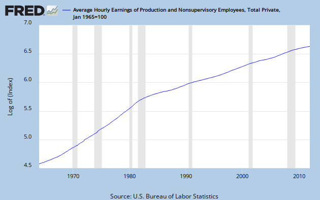
Here is a look at average hourly earnings, the typical income of a working stiff, presented on a log scale.

Like almost every time series you can imagine, including GDP, it exhibits a break near 1980.   The break is always to lower growth.  But, compared to most other data series, this break is especially sharp.

Hear is the same series compared to GDP, an approximate measure of the income of the nation, on a linear scale.  For this graph, each is normalized to a value of 100 in Q1, 1965.

While earnings have grown less than 8 times in 47 years, GDP has grown more than 20 times.

Clearly, the money has not gone to compensation of the workers whose labor actually creates the wealth of the nation.  That might explain some of the alleged envy.   (end update)

CORPORATE PROFITS

As a first step in finding where the money has gone, let's consider the growth of corporate after-tax profits since about 1950.  You can see it in this FRED graph.   It's on a log scale, so constant growth would be a straight line.  There are lots of wiggles, but I see an increasing slope over time, and it's not an optical illusion.

There are a lot of ways to parse this.  One is to connect the dip bottoms with straight lines.  I've done that with alternating red and blue to show the slope increasing over time.  The problem is selecting which bottoms to connect.  Some alternate choices are indicated in yellow.  The yellow lines define times of above normal profit growth: 1970 to 1980, 1986 to 1998, and 2001 through 2007.  Each of them leads to a correction, indicated by a purple line across the top of the decline.

After I did all that, it occurred to me to let Excel throw an exponential best fit line on the data set, and you can see that as well.

I see now that I could have included another yellow line from 1961 to 1967.  Notice that with each yellow line, the data set advances above the exponential best fit line before a sideways correction takes it below again.  After the correction is complete, profits increase again until the best fit curve is breached.  Or, they did until now.

Remember that on a log scale constant growth rate is represented by a straight line, and that the growth compounds, so that the underlying increase is exponential.  Sooner or later, that has to end.  Nothing in the real word can go to infinity.  Here we see an exponential curve on a log scale.  This demonstrates an increasing growth rate.  Therefore, the underlying increase is greater than exponential.  If exponential growth is unsustainable, what would you say about greater than exponential growth?

In fact, the whole trend might now be falling apart, as the last blue line has a much lower slope.  Also, for the first time following a correction, profits have stayed below the trend line, and the gap is increasing.

To show the extent of national income capture by corporations, here is a graph of corporate profits as a percentage of GDP.   I've divided the set into two segments: 1951 to 1979, and 1980 on, and had Excel place a linear trend line on each.  This division is somewhat arbitrary, but almost every economic time series you can find has a break point within a few years of 1980.  Division between '79 and '80 is the least favorable to my point that Profits/GDP had no trend in the post WW II Golden Age, but have trended sharply upward during the Great Stagnation period.

Profit/GDP growth was unusually poor from 1980 through 1986.  Then from late 2001 through early 2006 it exhibited the greatest growth ever.  But remember the denominator effect.  Nominal GDP growth increased rapidly following the '80-'82 double recession; while GDP growth in this century has been generally slow.  The financial melt-down of 2008 caused a dip that was sharp and brief, but the rebound has not gone to a new high.  But even now, in the midst of anemic recovery, profit/GDP is hovering in the 9 to 10% range, far above historical norms.

CONCLUSION

The corporate profit growth picture looks unsustainable, and that is troubling.  What it means for the future is anybody's guess.  But, what we get from it is the first partial answer to the question, "Where has all the money gone?"

Gone to profits, everyone.

1/17 Update:  Cross posted today at Angry Bear.

Fed Policy Failure As Root Cause

I decided long ago to not read Scott Sumner, but I'm not bigoted about it.  Karl Smith directs us to this post by Sumner, in which he does a clever personal riff on a Wittgenstin quote.

In the context of the great recession we are still enduring, Sumner uses this to blame the Fed.  He says this in comments to his post, at 14:13 on 16 Dec,. re: the Fed.

 They intervene every second of every day. They control monetary policy and hence NGDP. 

And this:

The crisis of 2008 was caused by tight money at the Fed. They deviated from their normal dual mandate in September 2008, and it was all downhill from there.

There is probably a good argument that the Fed was following tighter policy than they should have around that time - and quite possibly had been for a considerable while.  But the view that monetary policy is omnipotent seems awfully one-dimensional to me.  I cite the inability of QE money to spur the economy - it has mostly wound up in excess reserves. This view also implicitly dismisses the idea suggested about 20 minutes earlier by commentor Donald A Coffin, that capitalism has some level of inherent instability -- which Sumner simply shrugged off.

The idea that that the Fed is intervening during seconds, hours, days and weeks on end, when they make no policy decisions at all seems to be a reach too far.

The really striking thing, though, is the accusation that that the Fed made a policy turn in September, 2008.  Does anybody have a clue what they might suddenly have started doing differently?

Later in comments, flow5 says:

That’s not exactly what happened. Bernanke tightened MVt for 29 consecutive months. The Case Schiller housing index peaked @189.93 when Bernanke initiated his tight money policy. Based upon the FED’s technical criteria (interest rates), the 4th quarter contraction in 2008 was already “set in stone” beginning in Jan of that year. I.e., the Fed’s failure to prevent NGDP from falling started long before the economy collapsed.

In the midst of all this, what I find most puzzling is Sumner's insistence that a market in NGDP futures contracts will lead to stable levels of NGDP.  This is the highest order of dog wagging I have ever seen suggested to any tail.

A Different Look At The Great Stagnation - Pt 2

For part 1, see here.

THE GOLDEN AGE AND THE GREAT MODERATION

The golden age was a period of strong, but sometimes erratic, economic growth.  To illustrate this, consider the quarterly rate of change since 1947 in gross domestic product (GDP.)   GDP is an aggregate measure of all the goods and service produced in the country.  It’s not perfect, but it is a reasonable barometer of the state of the economy, and growth rates tell you where it is headed.  The Bureau of Economic Analysis (BEA) provides relevant data in many forms.  Graph one is a data plot of quarterly percent change from the preceding period in real (inflation adjusted) GDP, seasonally adjusted at annual rates, from BEA. This plot is color-coded by presidential administration, blue for Democrats, and Red for Republicans.  As you can see, this number jumps around a lot, but less so in recent decades.  Also shown are the average values for all data from 1947 through 1980, 3.73%, in green, and the average from 1981 through the first quarter of 2011, 2.81%, in red.  Note that since 1981, average GDP growth has been almost a full percentage point lower than it was during the Golden Age.

Also shown is an 8 year moving average in yellow.  I chose an 8 year span for the moving average to smooth out over the length of a two-term presidency, but any long moving average will tell the same story. Until recently, the lowest dip in that (moving average) line bottoms out at 2.35% in 1982, and the highest bottoms out 2.71% in 1986, with no particular pattern across time.  The lowest bottom of all occurred in the recent Great Recession, bottoming out at 1.54% in the second quarter of 2009.  The dramatic change is in the tops. After a broad double peak from 1966 to 1969, topping out at 5.39% and 5.29%, the remaining peaks are between 3.99% and 4.07% - scarcely above the golden age total period average.  The other notable feature is the steady decline in quarterly data peaks throughout the G. W. Bush administration and the corresponding slide in the eight year average, culminating in the crash of 2007.

Figure 1

During the Great Stagnation, the reduced volatility in the quarterly GDP growth numbers appears in the graph as generally less severe bottoms, and even more dramatically as less expansive tops.  The degree of volatility can be precisely determined using the statistical technique of standard deviation.    The next graph shows how the standard deviation has changed since WW II.

 Figure 2

The blue curve is the standard deviation (Std Dev), based on the previous 34 quarters.  We’ll get to the red line later.  Sure enough, the Std Dev falls over time, as the blue best-fit trend line confirms, but it does not fall monotonically.

How can we account for this?  In the 50's, there was economic turmoil, as the economy restabilized during the first wave of the baby boom, and about 7 million soldiers reentered the work force following WWII - which came hard on the heels of the Great Depression.  This was a dynamic time, with wild growth peaks in 1950, '52, and '55, along with recessions in 1953, '58, and '59-60.  Then came the First Little Moderation  - a decade with steadier GDP growth and – most significantly, no recessions until late in 1969.   The 70's brought stagflation, the end of the Viet Nam war, and another series of wild gyrations in GDP growth - though, except for one spike in 1978, and the recession of 1980 - not as wild as the '50's. Reagan's high spending and deficits held recessions at bay after 1982, and volatility began to decline a few years later.   After a modest peak in late 1987, GDP growth declined as well, and the resulting recession contributed to denying George H.W. Bush a second term.  The Clinton administration gave us relative prosperity, along with the Second Little Moderation – another multi-year span without a recession.  Volatility remained steady at a low level throughout his two terms, before dropping further to an all-time low in 1999.  Despite this, his policies were too conservative to rekindle anything like a golden age. By 2000, the wheels were about to come off the Clinton boom anyway, but the grotesque economic policies of the George W. Bush  administration threw us farther over a deeper cliff than was necessary.  His profligate spending made Reagan look prudent, and gave us an anemic and declining series of GDP mini-peaks, culminating in the crash of 2007.  Barack Obama’s administration has not been able to foster significant growth and a robust recovery while dealing with a Congress dominated by blue dog Democrats and overtly obstructionist Republicans.  It’s particularly interesting that the recent Great Recession barely registers as a blip on the blue line.

Which brings us to the red line in Fig 2: relative standard deviation (RSD), determined by dividing the standard deviation by the average of the same 34 data points, here multiplied by 3.5 to put it on the same scale as Std Dev.  Part of the reason that the Std Dev became smaller over time is that the numbers used to calculate it were smaller. To this extent that this is operating, the Great Moderation is a meaningless data artifact.  However, if this were strictly true, the best fit line for RSD would be exactly horizontal.  It’s not, but it does have a smaller slope than does the best fit line for Std Dev, so the idea is not totally without merit.  Let’s have a closer look.

By the end of the first Little Moderation, RSD dropped to a level below that of most of the Great Moderation.  It then rose slightly, was stable from ’71 to ’73, and took a big jump with the recession of ’74.  After slipping over the rest of the decade, RSD shot to an all time high during the recessions of ’80 and ’82.  The big drop occurred between ’87 and ’90, and the low level was maintained until the Great Recession.

Volatility is the intensity of variability.  Big changes in short time spans register as volatility, causing Std Dev and RSD to increase.  As figure 1 shows, the biggest variations come from recessions and quick, strong recoveries.   There were three recessions in the 50’s so RSD never had a chance to decline.  The 60’s and the 90’s were both recession-free, so RSD could decline in the one case, and stay low in the other.  The recessions of the 70’s were deep, but the recoveries were strong, so volatility climbed.  The back-to-back recessions of ’80 and ’82, with sharp recoveries in ’81 and ’83 took RSD to an all-time high.  The Great Recession propelled RSD back up to a level not seen since the 80’s.  Simply, all of the volatility jumps can be explained in terms of recessions.  Avoid recessions, and Std. Dev. will be low.

How, then, do we explain the two Bush administrations, with their recessions in 1990 and 2001, but no jump in volatility?  In each case the fall into recession was not sudden – it followed several months of low or declining GDP growth.  Similarly, in each case, the climb back out of recession was slow, faltering, and failed to generate even a single quarter where GDP growth topped 7%.  In contrast, from WWII until 1983, top recovery quarters typically exceeded 10%.

What this indicates is that the Great Moderation really is a data artifact – though not quite in the way I expected.  Reduced GDP growth numbers play a part, but the real key is understanding how recessions contribute to observed Std Dev.  Recession-free times have low Std Dev values, and tepid recoveries from recessions that occur in a low growth context will also have low values.  While the Great Moderation is real, the standard explanation is inadequate, and comes from failing to look at the data with a critical eye.


________________________________________________

This was intended to be a chapter in a multi-author book project.  The project fell through for reasons not related to the project itself.

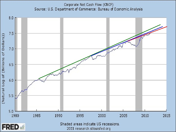
Corprate Net Cash Flow

Connecting peak to peak a la Krugman, since 2005, CNCF seems to have established a new trend line (red) at slightly lower slope than the trend line from the late 90's (blue.)  This, in turn, has a lower slope than the previous trend line (green) from about 1985. 

You'll have to believe me when I tell you a few historical facts (or go to FRED and look them up yourself.)  First, the green line slope is virtually identical to that from 1950 through the early 1970's.  Second, the slope from the late 70's through '85 was greater than the green line slope (you can see that in this chart if you look to the left.)  Third, the slope through the mid 70's was greater still.

Restated, the growth of CNCF has never been slower in the post WW II period than it is right now.  Yet Karl Smith is excited about current growth, is making optimistic predictions about 2012, and expects inflation.

My comment:

What they miss is that labor’s share of national income will fall and probably at a slightly faster pace than before the recession.

I am one who so objects, and I certainly haven’t missed it.

http://jazzbumpa.blogspot.com/2011/06/labors-share.html

How can increasing corporate profits, per se, be inflationary? This just enables even greater wealth disparity. A falling labor share means most people get squeezed out of buying discretionary items. Hence, a continuing (and increasing?) aggregate demand shortfall,

I’d love to see a detailed explanation of how inflation can increase in this scenario.

BTW – put your graph on a log scale and you’ll see your CNCF/GDP ratio climbing during recessions, and very dramatically during this last one. Such was not usually the case before about 

1970 (recession ca. 1955 is the exception.)

http://research.stlouisfed.org/fredgraph.png?g=3yb

Also, beware the denominator. Progressively lower GDP growth since ca. 1980 skews your ratio upward.

http://research.stlouisfed.org/fredgraph.png?g=3yd

JzB

Karl and I can't both have it right. Which of us do you think is wrong, and why?

We Are Poorer than We Should Be

Reading this post at Tux's reminded me of something I wrote for a project that will probably never see the light of day in its originally intended form and format.

Here, then, is the opening of what was intended to be a chapter in a book.

Part 1.

A DIFFERENT LOOK AT THE GREAT STAGNATION

Anyone who believes exponential growth can go on forever in a finite world is either a madman or an economist.

– Kenneth E. Boulding

It's no secret that the general economic environment in the U.S. has changed dramatically since some poorly defined moment within a few years of 1980. The dramatic decrease in the volatility of aggregate economic activity is commonly known among economists as The Great Moderation. The traditional view (circa 2005) was that this is a good thing, resulting from the absence of energy price shocks, improved monetary policy, and better inventory management techniques. This interpretation looks pretty hollow in the wake of the 2007 recession, when the economy collapsed, monetary policy was reduced to relative impotence, and energy price shocks are again dominating the economic landscape.

My view is that the volatility reduction is the result of a gradual decline in economic health over that time period – what skeptics like me call The Great Stagnation. In fact that is the title of a recent e-book by George Mason University economist Tyler Cowan.

I'm a bit on the skeptical side of agnosticism regarding Cowan's main point – that we have run out of low hanging technological, financial, and resource-based fruit.  The technology claim, if it has any merit at all, might be an artifact of a slow down in government spending at all levels – coincidentally, also since about 1980.  I’ll let those with more specialized knowledge sort out the rest of Cowan’s claim. My position is that, while Cowan's argument might (or might not) have some intrinsic value, it largely misses the point.

More on the mark is Cowan's corollary – that we are poorer than we realize. He thinks measurement techniques currently in vogue overstate our wealth. While this may be true, there is plenty of data available to demonstrate in directly measurable ways that, in the aggregate, we are poorer than we should be. And what makes this even worse is that growing income and wealth disparities have led to an economically top-heavy society that is probably unstable. Ultimately, this will require either effective mechanisms to redistribute wealth downward, or effective mechanisms to repress an increasingly impoverished and unruly population. The latter could be accomplished by a stark and impenetrable stratification of society into haves and have-nots – the kind of forced repression that leads to either South American style banana republicanism or 12th century European style feudalism.  On the other hand, forced redistribution led to America's post WW II golden age.

I have not been a long-time observer of the deterioration of the human condition, so I did not have a keen view of the long, slow slide that has been taking place since the post WWII golden age ended.  My awakening came with the impeachment of Billy-Bob Clinton, our first Bubba President.  This, for me was a real WTF?!? event.  To say there was no there there is to wildly overstate the significance of Clinton's history of dalliances with various consenting adults.

With my eyes thus opened, I watched the election appointment of The Shrub with a combination of horror and disgust.  His plan to ruin America by going to war while simultaneously cutting taxes was a success that even Grover Norquist would have had trouble hoping for.

And now we have some significant minority (oh god, please let it be no more than that) of the American people openly embracing a rouge's gallery of even worse Rethug presidential hopefuls. People who cheer for Herman Cain's claim to be a surrogate Koch brother, and increase their donations in the light of his sexual harassment revelations. 

The intellectual nihilism of conservatives is perfectly demonstrated by Shrub, Cheney, McCain, Cain, Bachman, and most especially by the idiotic Rick Perry.   You see, it takes anti-intellectualism, ignorance or outright dishonesty to embrace the Rethug policies of upward wealth redistribution, and all that they imply.

I am seriously fearful of the world we will hand to my grandchildren - now aged from 4 to 14.  We are on a road to to deep repression or revolution, and eventually, perhaps, even another World War.