Unhealthy Inequality

This is from 7 1/2 years ago.

Imagine how much worse things are now.

Income inequality Over Time

Some people think that other people, like Krugman, Piketti, Saez, and - well - me have it all wrong about income inequality. I might take a deep dive into that link at some future date, but for now here are quick graphical looks at reality.

I plotted data from the Census Bureau Historical Household Income Tables to get these graphs.

First, here are the upper income limits for the bottom 4 quintiles, along with the lower limit for the 95th percentile for years from 1967 through 2017.

Graph 1 - Income limits per population slice

Clearly, the spread between quintiles has increased, and by larger amounts as you go up the income ladder.

Looking at it in constant 2017 dollars in Graph 2 makes this picture even more stark.

Graph 2 - Income Groups in Constant 2017 Dollars

The modest nominal gains in the bottom two quintiles have been largely obliterated by inflation. The spread between groups has widened.

What is the mechanism for increased disparity?  The data shows that it is income captured by each group.  This is presented in Graph 3.

Graph 3 - Aggregate share of income

Even into the 4th quintile, the aggregate share of each lower group has declined, while the top quintile has captured more than 100% of the gains, almost every year over the last 50 years.

Graph 4 shows the 1st and 4th quintiles along with the top 5%.

Graph 5 - Including the Top 5%

The top 5% have gained a significantly increasing share of the pie, and now are receiving about as much as the entire 4th quintile.  The pie is growing, but the rich are taking an increasingly larger slice.

I haven't taken a hard look yet at the article I linked at the beginning of this post.  We'll see what kind of arguments are put forth to counter the reality I have presented here.
.

Effort and Reward

Jim Kwack cites Milton Friedman with the idea that inherited wealth should be taxed at the same rate as regular income.   Given a modest exemption - say a few million dollars, to avoid destroying family businesses - I concur.

I'm not sure I believe Friedman when he says this, though.

The man who is hard working and thrifty is to be regarded as ‘deserving’; yet these qualities owe much to the genes he was fortunate (or fortunate?) enough to inherit.”

This deterministic idea gives the individual no credit at all for his own hard work and dedication, and implies that twins should be equally hard working and "deserving."  Even more insidiously, though, it enables thinking about the unsuccessful in terms of a stereotyped notion of hereditary laziness for those inheriting less fortunate genes.  Down that road lies eugenics.

The lucky sperm club notion does have merit, though.  Not in terms of abilities but in terms of financial stability and backing, educational opportunities, network connections, access to health care and numerous other intangibles.

I have a different take from Friedman, more along the lines of the ideas expressed in comments to Kwack's article by Charles Broming.   Luck - and not of the genetics dice-roll type - plays a huge and generally unrecognized roll in the success or failure of any endeavor.  Two identically talented and ambitious entrepreneurs can set up identical businesses on the same day and one might succeed while the other fails due to either completely random factors like the weather, a change in traffic patterns or gentrification, or some other uncontrollable external factor; or due to unequal opportunities like available financing, suitability of location or a variety of other luck-related circumstances.

Two identical baseball pitchers can have widely different results due to the park they play in, the quality of the defense behind them, and the run support given by their own offense.   This barely hints at the notion of unequal opportunities.

Beyond that, there is the fact that rewards are not distributed linearly with respect to outcomes.  In fact, reward levels can often be quantized.  This, from the world of pro golf, is illustrative.

The difference between making it back onto the tour and being demoted to the Nationwide might only be a couple of dozen golf shots over the course of a season, but the financial repercussions are huge. Prize money on the Nationwide is only about 10% of the tour’s. Last year’s top moneymaker on the PGA Tour, Luke Donald, made $6.7 million on the golf course; the top player on the Nationwide Tour made $414,000. Most Nationwide events are not televised, and endorsement deals are one-third as big, if not smaller. If playing on the PGA Tour is like having your product stocked at Wal-Mart, competing on the Nationwide is like selling through a regional supermarket chain.

I firmly believe that a more equal society is, generally speaking, better than a society characterized by stark and growing inequality.  Whether this notion is supported by brute economics or not; a humane consideration of quality-of-life issues for the have-nots influences the equitability and stability of society in numerous non-trivial ways.

All of this lends support to my belief in high inheritance taxes and a steeply progressive income tax.

We don’t let gravity keep us from building bridges.

Steve Randy Waldman, while talking about the economics of inequality, mentioned in passing that the poor die with negative wealth.

Doesn’t this imply that their spending needs were greater than their ability to spend?

Doesn’t that suggest that if they had a little more, they would spend every penny of it?

Nor does it have to be technology driven. Maybe they get a third meal one day a week, a better pair of shoes for the kids or a new pair more often, a five-year-old instead of a seven-year-old used car.

Still – the economic and the moral considerations converge at the low income level. It’s true that economics is not a morality play. However well or ill we understand it, econ, as a natural phenomenon, is a brute force, like gravity. That’s why humans with a moral compass need to intervene. We don’t let gravity keep us from building bridges.

Revolting

Image Source

But when the revolution does come, the 1% will have the tea party on THEIR side.

And them @$$ h0lz has gunz.

We're screwed.

Middle Class Melt

Since I got preempted posting the inequality video at AB, I thought I'd offer this as a follow-up.

H/T to Rachel Maddow.

Inequality

Last night, Rachel Maddow showed a graphic similar to what is seen early in the video presented below.  It indicated what the vast majority of Americans think the ideal wealth distribution should be, and what they perceive the actual distribution to be - a considerably more skewed condition.  It also shows the reality, a condition far, far removed from the perception

The data Rachel presented is a stacked horizontal bar chart, essentially a one-dimensional representation.  The video shows this, and then follows up by presenting the data in another way, which is much more dramatic and effective.  Have a look.  It's well worth 6 1/2 minutes of your time.




This makes me wonder again how we compare in A. D. 2013 with the stratification of society in, say, A. D. 1213.   Now, the bottom 40% have essentially zero wealth.  That might have been true then, as well, and perhaps reaching for a couple more quintiles - for in those days the middle class had not yet been invented.  But at the top now, the distribution is so skewed that the 99th percentile have vastly more than the 98th percentile who have vastly more than the 97th.    

Don't get me wrong, those in the 97th percentile are doing very well, indeed.  But the top percent, and the top tenth of a percent in particular really have amassed wealth beyond the dreams of avarice.

Back in A.D 1213, could there possibly have been orders of magnitude differences among fine divisions of the top couple of percent?  In a time when wealth was measure in land, cows and gold chalices, that's very hard for me to believe.

I believe the corrective actions are very clear, and simultaneously politically impossible to implement.

1 Steeply progressive income tax structure
2 Steeply progressive inheritance tax structure
3 Stringent regulation, most especially of the finance industry
4 Break up the to-big-to-fail banks
5 Limit banks along State borders
6 Tax capital at a higher, not lower rate than labor
7 Increase the minimum wage to something livable
8 Increase earned income tax credits
9 Simplify the tax code in ways that encourage keeping jobs here
10 Create strong disincentives for off-shoring
11 Repeal Taft-Hartley and strengthen labor unions
12 Break up monopolies

Feel free to expand the list in comments.

If this looks a lot like the New Deal, that's not much of a coincidence.  The only time we ever had a robust middle class was in the years when New Deal policies were followed.  The systematic dismantling of the New Deal [call it the Raw Deal if you wish] has resulted in the erosion of the middle class, further impoverishment of the poor, and the vast enrichment of the already very wealthy, at everyone else's espense.

H/T to nanute who pointed me to this article where I found the video.

What is the Economic Middle Class?

My lovely wife shared this link with me on Facebook.  I got into a discussion in comments there with a right winger who suggested that $250,000 was a very reasonable estimate for median income in Boston.

As it turns out, median household income in Boston is $51,914, close to the national average, and way below the Mass. State average of $67,950.  But right wingers live in a data-free world, so this is no surprise.

Another contention in comments at that site is that the middle class is undefined and undefinable. Not so.  I define middle class household income as the middle quintile.  This range includes the median and a band around it wide enough to hold 20 percent of the population.  You might wish to concoct your own definition with a wider spread, but you'd better not be asymmetric around the median.  Feel free to use the middle three quintiles, if that is your preference.  But if your of concept of middle class gets very far beyond 50% of the population, you really ought to give more thought to what the word "middle" actually means.

Thinking about all this prompted a look at the various income quintiles.  The data, through 2009, is available at the Census Bureau web site, table 694.  This table provides historical data from 1967 through 2009 on the top income limit for the bottom 4 quintiles, and the bottom income limit for the top 5%, expressed in constant 2009 dollars.

Graph 1 presents this data.  The 3rd quintile - my definition of the middle class - is between the orange line and the yellow line.

In 1967, the threshold for the middle quintile was $32, 848.  By 2009, it had increased by 17% to $38,550.  This is a compounded annual growth rate of 0.38%

In 1967, the top limit for the middle (and threshold to the 4th) quintile was $46, 621.  By 2009, it had increased by 33% to $61,801. This is a compounded annual growth rate of 0.68%.

The threshold value for the fifth quintile increased from $66,481 in 1967 by 80% to exactly $100,000 in 2009.  This is a compounded annual growth rate of 0.98%.

To reach the top 5% required an income of 106,684 in 1967.  By 2009, this had increased by 69% to $180, 001.   This is a compounded annual growth rate of 1.25%.

So my comment sparring partner and the current presidential challenger he seems to support are a bit off base.  $250,000 in household income puts a family well above the 95th percentile.  In fact, that is just enough household income to crack the top 2%.

My ongoing hobby of debunking right wing nonsense aside, the point of this post is mainly to inform.
There are two main observations:
1) While the bottom two quintiles haven't changed much over the decades, entry to the third quintile has crept up a bit; and into higher categories it's moved up a lot.  We recognize this as stagnation in the bottom half and growing inequality in the top half, skewed powerfully to the top.
2) This data set stops in '09, so Obama is outside the discussion.  But we can see that all the way up to the 95th percentile, income growth was dead flat during the Bush administration.  No wonder the 95% percentile feels so poor.

But -- surely, some wealth was generated during those 8 years.  GDP growth was positive at least some of the time.  I wonder where it all went?

What the Hell?!? Friday - "Romney Girl" Edition

Via the Ed Show on FB or ABC News.

H/T to the LW.

Another Look at Wealth and Consumption - Pt 2

Correlations and Slopes Over Time

In Part 1, we looked at the ratio of consumption spending to net worth, and how it changed over time.  This time we'll look at the correlation between net worth and consumption.

Here is the big picture: personal consumption expenditures (FRED Series PCE) plotted against Net Worth (FRED series TNWBSHNO) Data is per calendar quarter.

Graph 1  Consumption vs Net Worth, 1959 - 2011

The data set is divided into two segments, with a break point at the beginning of 1997, with net worth at $30,315 and consumption at $5,467.  In a close up view, there is a clear slope change there.  Still, the selection is a bit arbitrary, since the high point of Q3, 1994, could also have been chosen, with net worth at $25291, and PCE at $4856.  But that is a detail, and no other reasonable breaks stand out.

Notably, both the slope of the data line and R^2 are significantly less after the break.  Visually, it's obvious that in the later data, there is a lot more scatter.  Also note that that big data moves post 1997 return to the continuation of the best fit line, pre-1997.

Slope and R^2 measurements for the entire data set and the two segments are presented in Table 1.  These numbers were generated using the linear trendline function in Excel.

 Table 1
 

Not so visually obvious are the declining slopes during the earlier portion of the data set.  Table 2 presents the same characteristics for data chunks of approximately 20 year duration.

Table 2


We saw in part 1 of this series that the relationship of consumption to net worth was not stable, so this result is not surprising.  And we can now see that as net worth increases, the sensitivity of consumption to increasing net worth decreases.

I can think of two contributing factors.  As wealth increases, the need to spend on basic necessities captures a smaller portion of that wealth, so the propensity to spend decreases.  I'll defer consideration of the other factor for now.

Here is a detailed look at how the slope of the PCE vs net worth line varied over time.  Graph 2 shows the 34 quarter slope values for the data points of graph 1.  The slope is plotted in dark blue, with certain time spans highlighted in contrasting colors: recessions are in orange, and the stock market and housing bubbles are in yellow.

Graph 2 Slope of Consumption vs Net Worth

Observations:
1) Except for the bubbles and the spike in the post-bubble recession of 2008, the values are mostly contained between a low of 0.168 and a high 0.246.
2) There was an upward trend that ended in the mid-70's, underscored with a blue line.
3) Values after the mid-70's, including the two bubbles, are contained in a down-sloping channel, outlined in green.
4)  Except for the early 80's and 90's events, recessions are marked by sharp, temporary slope increases.
5) The average slope is 0.184, with a standard deviation of .038
6) The bubbles highlighted in yellow in Graph 2 correspond exactly to the data points in Graph 1 that fall below the red best fit line.
7) The post-bubble recessions brought the slope back into the range described in Observation 1.  This is illustrated in Graph 1 by the returns to the blue best fit line.

If the normal relationship between net worth and consumption is described by a slope in the range of around 0.17 to 0.25, what is there about bubbles that causes drops into the range of 0.11 to 0.12 at the peaks?  I think the answer is the second factor that I defered until now.  The stock bubble and the housing bubble represented wealth increases that were not shared equally across the population.  Specifically, as I pointed out earlier, these assets are mostly owned by the richest population segment, and growth in wealth has excessively favored the top 1% of the population.   They have the least propensity to spend, and this tendency drives the PCE slope into the low range.

This FRED graph illustrates the point in a different way.

Graph 3 PCE, Net Worth and Disposable Income

There are four lines, Net Worth in green (divided by 5 to put it on the same scale); Disposable Income in purple, PCE in red, and Disposible Income multiplied by 0.931 in blue.  Note that the last two overlap almost perfectly, as I also pointed out earlier (see link above.)

The conclusions I'm drawing are
1) Since the bubbles increased wealth in a highly skewed fashion, the relationship between average wealth and consumption broke down.
2) When the bubbles burst, the normal relationship between wealth and consumption reasserted itself.
3) The underlying cause is that during the bubbles the relationship between wealth and income broke down, and afterwards reasserted itself.
4) The relationship between disposable income and consumption is robust across time and most extraordinary financial events.
5) All the foregoing suggest that if wealth distribution were more even across the population (and thus more closely tied to disposable income,) then the relationship between wealth and consumption would be more robust.

Cross posted at Angry Bear.

Another Look at Wealth and Consumption - Pt 1

 Part 1 - Spending as a fraction of Net Worth

Tim Duy weighed in on the output gap debate - not my topic, but he presented this chart of net worth as a percentage of GDP.

Graph 1 Net worth as a Percentage of GDP 

That got me thinking again about the issue of whether consumption spending is determined by income or wealth. Specifically, if consumption is determined by wealth, there should be peaks in consumption corresponding to the dot-com and housing bubbles shown on Graph 1.  However, as Graph 2 shows, there were no such peaks.

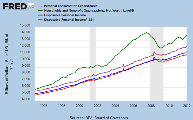
Graph 2 Personal Consumption Expenditures

I've argued already that, contrary to standard economic thought, consumption is directly determined by income.  (Posted at RB and at AB.) One observation was that consumption, as a fraction of income, didn't vary much over time, averaging 90.1% with a standard deviation of 2.1%. 

I took a similar look at consumption and net worth, data from Fred.  The next three graphs show personal consumption expenditures (PCE) as a decimal fraction of net worth (blue, left scale) along with net worth (NW) (red, right scale) over different time spans.

Graph 3A  Expenditures/Net Worth and Net worth, 1959-79,

Graph 3A spans from 1959 - the beginning of the data set - to 1979.  Net worth rises exponentially as the population grows.  Adjusting for population growth does not change the shape of the net worth curve, so, in the aggregate, we were becoming richer during those years.  Note that PCE/NW follows a generally similar, though far bumpier trajectory.  As I pointed out in the prior post, the personal savings rate also increased during this period, so the average worker was able to both save and spend more.

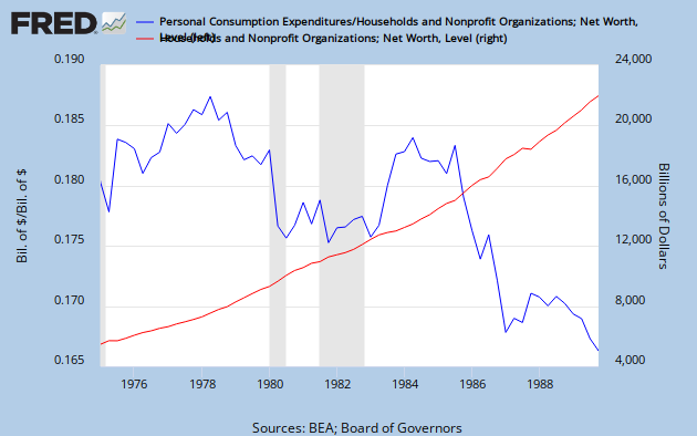
Graph 3B  Expenditures/Net Worth and Net worth, 1975-90

Graph 3B spans from 1975 to 1990.  Net worth continues on its exponential track.  But, after about 1979, PCE/NW drops, reversing the prior trend.  By 1990, PCE/NW is no greater than it was in the early 1960's.  Meanwhile, the personal savings rate also dropped - to a range below that of the early 60's.

Graph 3C  Expenditures/Net Worth and Net worth, 1989-2011

Graph 3C spans from 1989 through October, 2011.  The exponential growth of net worth falters before and during the two most recent recessions.  After about 1994, PCE/NW is a roller coaster ride.  Of particular interest is the exactly contrary motion at a detail level between NW and PCE/NW, after about 1998.  During the housing bubble of mid-last decade, PCE/NW hit an all time low.

What narrative makes sense of these three graphs?  Here's my attempt.

Through the 60's and 70's, the standard of living was increasing, as incomes and net worth rose together.  This allowed more discretionary spending, and therefore, the fraction of NW that was spent increased.

In the 80's, aggregate net worth continued to rise, but consumption spending, quite dramatically, failed to keep pace.  Lane Kenworthy has repeatedly pointed out that middle class income growth has decoupled from general economic growth as the upper income percentiles have captured an increasing slice of total income.  As the wealthy grew wealthier and the middle class fell behind, the fraction of NW that was spent declined - exactly the opposite of what should happen if increasing wealth determined spending.  But exactly what should happen if increased wealth is diverted to the already wealthy who have less of a propensity to consume.

During the 90's, growth in median family income and GDP per capita were close to parallel (see graph at the Kenworthy link)  so there was a lull in the decoupling.  For most of that decade, PCE/NW was close to constant at 0.18-.19.  But while spending was kept level, the personal savings rate continued to fall. 

During the current century, median family income has flat-lined, while GDP/Capita has continued to increase. The decoupling has resumed and the wealth disparity has widened.   During the two wealth bubbles, PCE/NW declined dramatically.  When the bubbles burst and net worth declined, PCE/NW increased  back into the 0.18-.19 range.  Most strikingly, from about 1998 on, the two lines in graph 3C exhibit exactly contrary motion at a detail level.

Conclusions:

There was a tight relationship between Net Worth and consumption through the 60's and the 70's, when earnings growth kept up with GDP and wealth disparity was slight by current standards.

This relationship broke down during the 80's - though one could argue as early as the mid 70's - as aggregate wealth and working class income decoupled.

Most recently, the relationship between NW and PCE/NW is inverse.  The big swings in NW that the bubbles provided also demonstrated that consumption spending does not depend on net worth.

As I indicated in the earlier post linked above, consumption spending does depend on disposable income, throughout the entire post war period.  A simple look at readily available data casts grave doubts on the idea that wealth, and not income, determines consumption spending.

UPDATE:   For the longer perspective, here is the data of Graphs 3 A-C on a single graph.

 Graph 4  Expenditures/Net Worth and Net worth, 1959-2011

In part 2, we'll look at how spending and Net Worth correlate.

Cross-Posted at Angry Bear.